2026-09-25
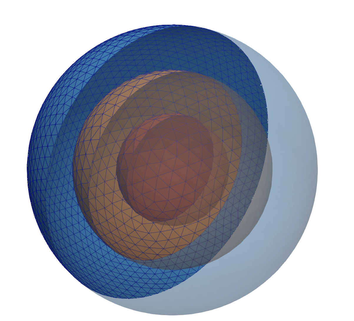
In this example, two concentric spherical shells with different
dielectric behaviors are considered. Moreover, on the innermost and
outermost spheres fixed potentials are applied. This constellation gives
rise to a simple analytic expression for the potential. In order to see
how to generate the concentricSpheres.yaml input file with
the preprocessor of POLARIS, check the
Preprocessor Tutorial.
| Parameter | Symbol | Value |
|---|---|---|
| Inner sphere radius | \(r_1\) | \(0.4\,\mathrm{m}\) |
| Middle sphere radius | \(r_2\) | \(0.7\,\mathrm{m}\) |
| Outer sphere radius | \(r_3\) | \(1.0\,\mathrm{m}\) |
| Inner dielectric permittivity | \(\varepsilon_{r1}\) | \(32\) |
| Outer dielectric permittivity | \(\varepsilon_{r2}\) | \(4\) |
| Inner sphere potential | \(V_1\) | \(100.0\,\mathrm{V}\) |
| Outer sphere potential | \(V_3\) | \(-50.0\,\mathrm{V}\) |
In order to compute the surface density and potential, run the command
polaris -i concentricSpheres.mesh -s concentricSpheres.yamlin order to obtain the result file
concentricSpheres.vtkhdf.
With
polaris.post -i concentricSpheres.vtkhdf -p concentricSpheres.xyz -s concentricSpheres.yaml the potential and E-field along a radial line are calculated and
tabulated in the file concentricSpheres.csv
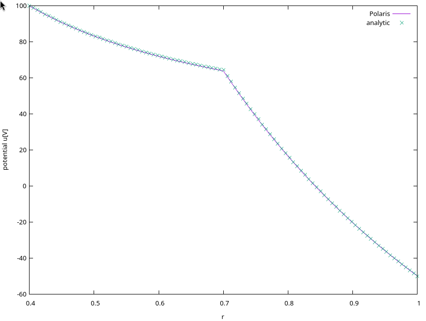
This problem with spherical symmetry can be reduced to two second-order ODEs in the radial direction. Their respective integration leads to solutions of the form
\[ u_1(r) = A + \frac{B}{r} \quad r_1 \leq r \leq r_2 \]
for the inner shell and
\[ u_2(r) = C + \frac{D}{r} \quad r_2 \leq r \leq r_3 \]
for the outer shell. The integration constants \(A\), \(B\), \(C\) and \(D\) can be obtained from the boundary conditions at \(r=r_1\) and \(r=r_3\), that is the prescribed potentials \(V_1\) and \(V_3\) and from the transmission conditions at \(r=r_2\). The final result of these constants can be found in the provided gnuplot script.
With the following commands
gnuplot
gnuplot> load 'concentricSpheres.gp'
one obtains a plot of the computed results along the radial line and the corresponding values of the analytic solution.
Below are screenshots from ParaView and the gnuplot image
|
|---|
| Surface mesh |
 |
|---|
| Potential along radial line |