2026-09-25
The geometry consists of a sphere with radius \(r=0.1\,m\) and a symmetrical biconical body with the same base radius \(r\) and height \(h=r\). The distance between the sphere and the tip of the conical body \(d=r/4=0.025\,m\). The conducting sphere has a fixed potential of \(V=100\,kV\), the potential of the conducting bicone is unknown.
In order to see how to generate the sphereBicone.yaml
input file with the preprocessor of POLARIS, check the Preprocessor Tutorial.
With the provided input files, POLARIS computes the electrostatic interaction between the two bodies.
By running the command
polaris --input=sphereBicone.mesh --settings=sphereBicone.yaml --output=sphereBicone.vtkhdfor, alternatively, the short version
polaris -i sphereBicone.mesh -s sphereBicone.yaml -o sphereBicone.vtkhdfthe computation is launched. In the terminal, the output should look like
#===================================================================
# INPUT
#-------------------------------------------------------------------
# Reading grid and settings ... done
# Grid with 1792 elements
#-------------------------------------------------------------------
# Mesh info
# Element type occurrences:
#     Tria6   :  1792
# Bounding box: [{-1.00000e-01,-1.00000e-01,-1.00000e-01} ---
#                { 1.00000e-01, 1.00000e-01, 3.25000e-01}]
# Mesh metrics:
#             Name Unit              Min     ID          Max     ID
#          Measure [L*L]          0.0001    512       0.0002   1546
#     Corner angle [degree]      43.8180   1280      86.0257   1280
# Condition number [-]            1.0042    575       1.7290   1280
#     Mutual angle [degree]       0.0004   1328      90.3316   1285
#-------------------------------------------------------------------
# Execution info
# Using 24 threads per rank
# Using 1 MPI ranks
# Input                         :    0.039s
#===================================================================
# CALCULATION OF SURFACE DENSITY
#-------------------------------------------------------------------
# Creation of calculator ... done
# BEM preparation               :    0.694s
#-------------------------------------------------------------------
# Computation of RHS ... done, |b| = 3577.7
# RHS computation               :    0.002s
#-------------------------------------------------------------------
# Solving main system ...
#-------------------------------------------------------------------
#    Iter           res
Sys      0         3.53343e-01
Sys      1         2.55590e-01
Sys      2         2.38317e-01
Sys      3         1.68034e-01
Sys      4         4.85218e-02
Sys      5         1.85809e-02
Sys      6         8.28103e-03
Sys      7         3.25397e-03
Sys      8         1.23608e-03
Sys      9         5.91779e-04
Sys     10         2.90968e-04
Sys     11         1.77854e-04
Sys     12         1.14345e-04
Sys     13         9.10840e-05
# System solver stopped with reason 'relative tolerance'
#           after 14 iterations, |x| = 3.99089e+00
# Solving                       :    0.035s
#===================================================================
# CALCULATION OF SURFACE POTENTIAL AND E-FIELD
#-------------------------------------------------------------------
# Solving system to compute normal E-field ...
#-------------------------------------------------------------------
#   Iter           res
EN      0         1.00000e+00
EN      1         4.38443e-13
# Solver for normal E-field stopped with reason 'relative tolerance'
#           after 1 iterations
# Normal E-field                :    0.002s
#-------------------------------------------------------------------
# Computation of surface potential ...
# Solver for potential stopped with reason 'direct solve'
#           after 1 iterations
# Potential                     :    0.001s
#-------------------------------------------------------------------
# Computation tangential E-field
# Tangential E-field            :    0.002s
#===================================================================
# POST-PROCESSING ...
#-------------------------------------------------------------------
# Electrodes
#-------------------------------------------------------------------
# Name              Appl. voltage     Total charge
  Sphere            +1.00000000E+02   +1.28700173E+02
#-------------------------------------------------------------------
# Floating potentials
#-------------------------------------------------------------------
# Name              Appl. charge      Voltage
  Bicone            +0.00000000E+00   +4.56739990E+01
#-------------------------------------------------------------------
# Dielectrics
#-------------------------------------------------------------------
# Name              Avg. voltage      Total charge
  Air               +7.75022862E+01   +1.28770181E+02
#-------------------------------------------------------------------
# Integral forces
#-------------------------------------------------------------------
# Name             Fx               Fy               Fz
  Sphere           -1.22436356E-11  -2.20701448E-11  +3.15753156E-08
  Bicone           -2.17481179E-13  -3.47305002E-13  -2.84802183E-08
  Air              +1.24611168E-11  +2.24174498E-11  -3.09509735E-09
  SUM              +0.00000000E+00  +0.00000000E+00  +0.00000000E+00
#-------------------------------------------------------------------
# Field extrema
#-------------------------------------------------------------------
  Range of potential: [ +4.56739990E+01 : +1.00000000E+02 ]
  Max of Eout field:     2.75194181E+03
  Max of Ein  field:     0.00000000E+00
#-------------------------------------------------------------------
# Post processing               :    0.039s
#===================================================================
# NORMAL TERMINATION
#-------------------------------------------------------------------
# Number of elements = 1792
# Total runtime                 :    0.815s
# Total memory consumption:
#       -- Peak memory per rank: 101.316MiB
#       -- Total peak memory:    101.316MiB
# Find VTKHDF file with solution data in
#    sphereBicone.vtkhdf
#-------------------------------------------------------------------
which indicates the four main sections of the analysis:
Additionally, with polaris.post the potential and the
electric field can be evaluated at all points provided in
sphereBicone.xyz by calling
polaris.post --input=sphereBicone.vtkhdf --settings=sphereBicone.yaml --points=sphereBicone.xyzor, alternatively,
polaris.post -i sphereBicone.vtkhdf -s sphereBicone.yaml -p sphereBicone.xyzThe generated terminal output should look like
#===================================================================
# INPUT
#-------------------------------------------------------------------
# Reading solution file, point cloud and settings ...
# Input                         :    0.002s
# Using 24 threads per rank
# Using 1 MPI ranks
#===================================================================
# FMM-BASED FIELD EVALUATION
#-------------------------------------------------------------------
# Preparation                   :    0.007s
# FNM setup                     :    0.017s
# FNM apply                     :    1.253s
#-------------------------------------------------------------------
# Field extrema
#-------------------------------------------------------------------
  Range of potential:   [ +3.34033683E+01 : +8.11624708E+01 ]
  Range of E-field(X):  [ -2.61726255E+02 : +2.61728129E+02 ]
  Range of E-field(Y):  [ -2.61724368E+02 : +2.61727410E+02 ]
  Range of E-field(Z):  [ -1.51320414E+03 : -3.72969881E+01 ]
  Max eField magnitude:    1.51320414E+03
#===================================================================
# NORMAL TERMINATION
#-------------------------------------------------------------------
# Number of evaluation points: 1089
# Total runtime                 :    1.283s
# Total memory consumption:
#       -- Peak memory per rank:  46.164MiB
#       -- Total peak memory:     46.164MiB
# Find CSV file with solution data in
#    sphereBicone.csv
#-------------------------------------------------------------------Both result files, sphereBicone.vtkhdf and
sphereBicone.csv can be post-processed with ParaView.
In the terminal output of the Main run one finds the block
#-------------------------------------------------------------------
# Floating potentials
#-------------------------------------------------------------------
# Name              Appl. charge      Voltage
  Bicone            +0.00000000E+00   +4.56739990E+01
We see that calculated floating potential on the bicone is
approximately \(45.674\,kV\) (note that
everything is in \(kV\)) and thus very
close to the results reported in [1]. The
full set of results can be found in the result file
sphereBicone.vtkhdf.
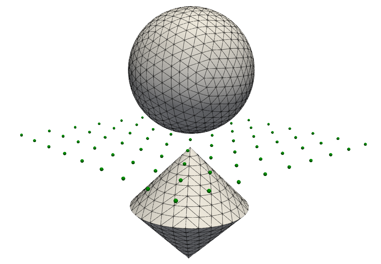
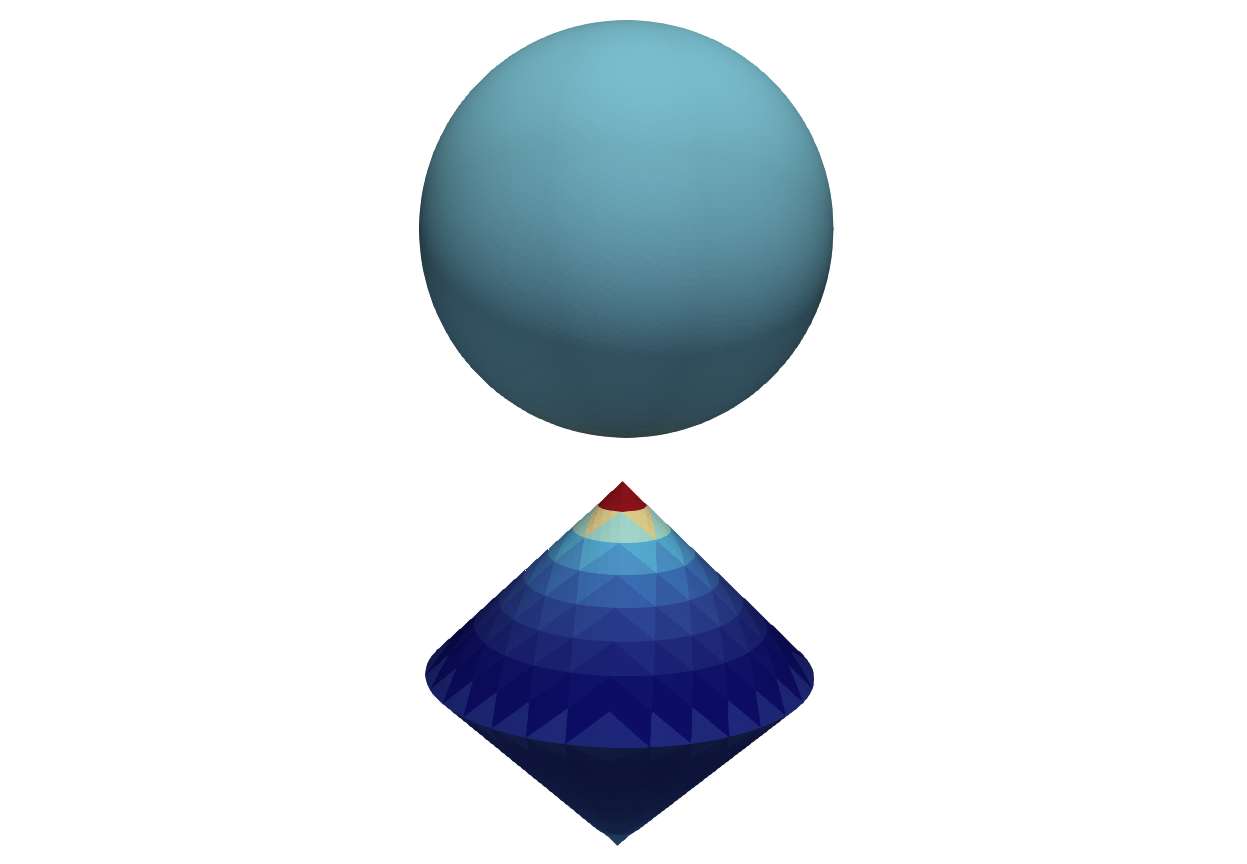
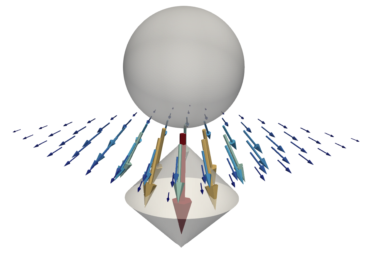
Below are some screenshots from ParaView that display the results
|
|---|
| Surface mesh and evaluation points |
 |
|---|
| E-field on the surface |
 |
|---|
| E-field at evaluation points |